
数字图像处理
第二章 数字图像基础
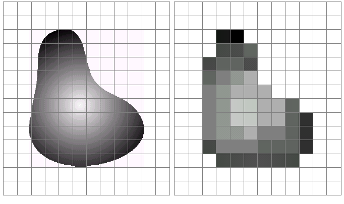
2.4 图像取样和量化
1.取样和量化基本概念
取样是空间离散化,量化是幅值离散化。
量化是将f(x, y)的连续分布的值划分为若干个字空间,在同一字空间内的不同灰度值都用这个空间内某一个确定值代替,形成一个有限可列数值序列。
显然,量化误差就是有限个离散值近似表示无限多个连续值产生的误差,也叫量化失真。
2. 数字图像的表示
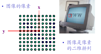
我们可以用双函数来表示像素,其中两个参数就是像素的坐标。
其中,M, N必须是整数,有时候将灰度的取值范围称为图像的动态范围,将占灰度级的全部有效段的图像叫做高动态范围图像。
存储数字图像的比特数为$b = M \times N \times k$,当一幅图像有$2^k$个灰度级时,则该图像是k比特图像。
比如黑白图像,有256个灰度级,即$2^8$个,$k = 8$。
空间分辨率:图像中可辨别的最小细节。单位:dpi(dots per inch)单位距离内的像素数。
灰度分辨率:灰度级中可辨别的最小变化。单位:bit,用于量化灰度的比特数。
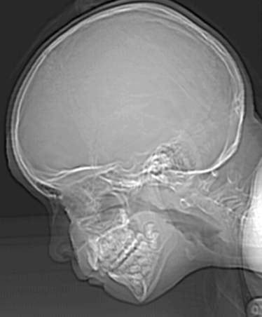
这是256灰度,而下图,是4灰度。
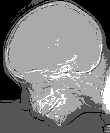
并且,对于大量细节图像,只需要较少的灰度等级。
4. 图像内插
即重采样。由已知像素数估计未知像素的像素灰度。
比如坐标关系:
词向量(Word2Vec)
简要来说就是把词汇用向量来表示,一般是行向量,每一列表示一个特征,通常想精确描述词汇所有特征,大概需要50-300维向量,这也是我们通常定义一个词向量的维度范围。但实际上向量是降维之后的结果,我们看到的经过降维的结果已经不能逐列分析其含义了。
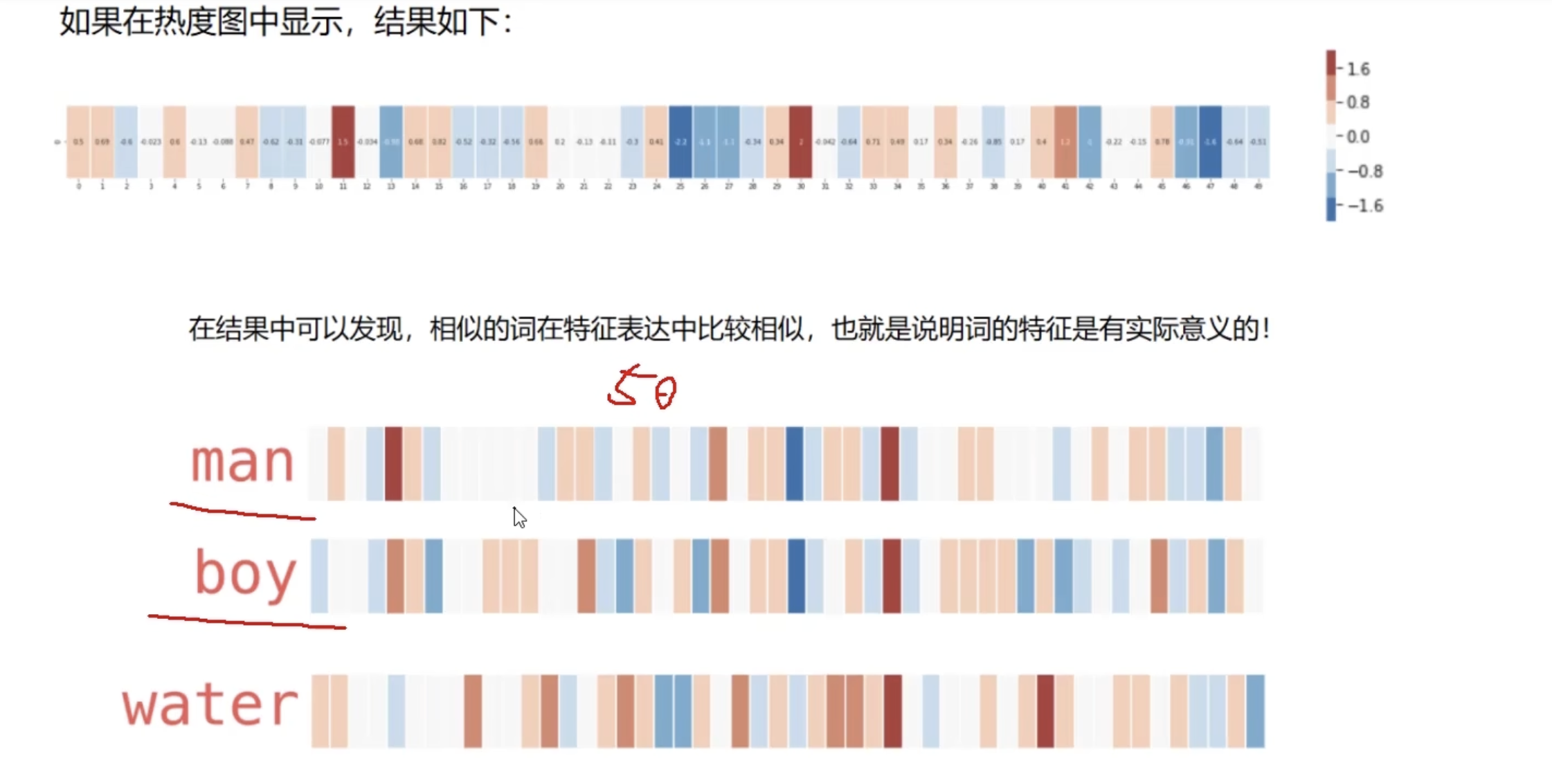
可以用热度图来表示词向量中每一项的大小。
实际上我们的RNN模型,应用于自然语言处理,就是想预测下一个词是什么,如图所示。
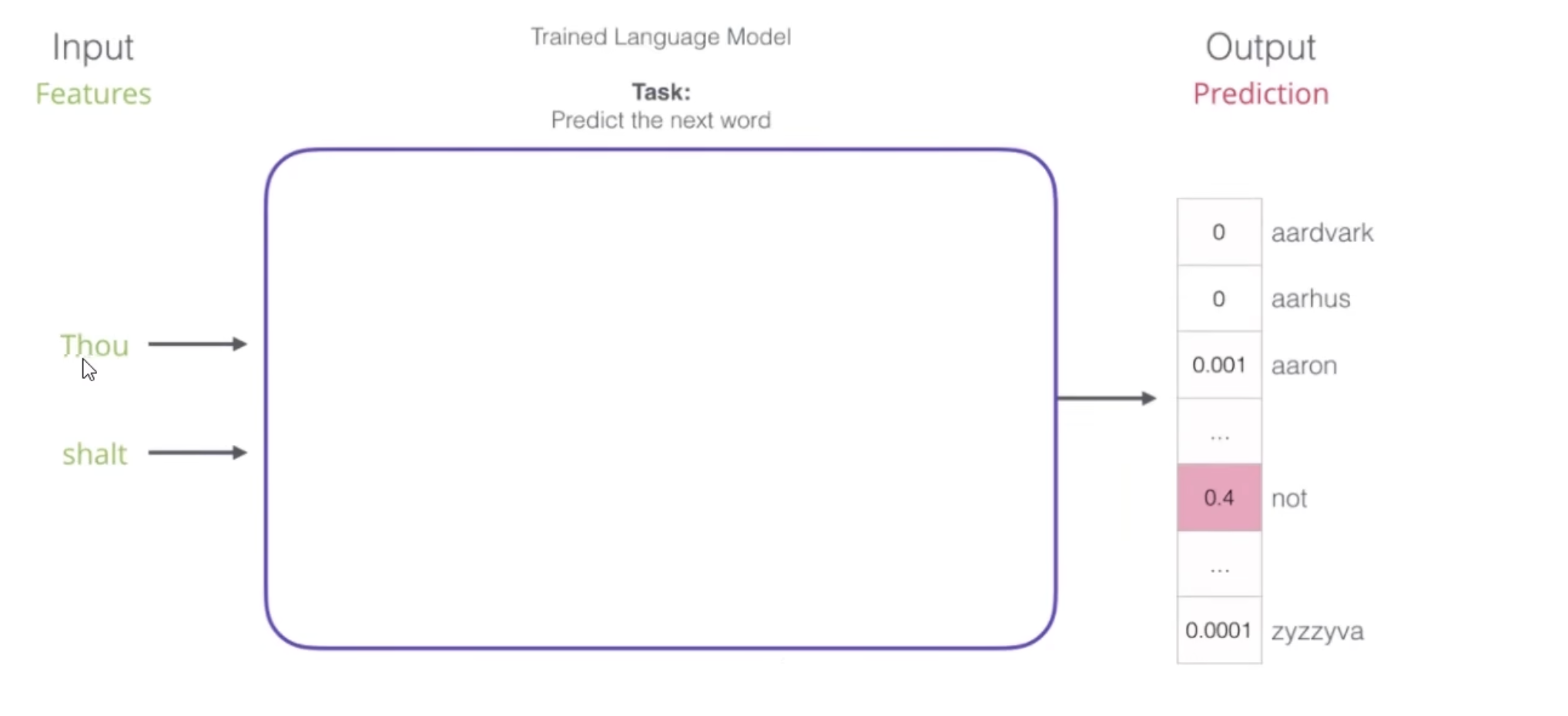
得到下一个可能得词汇的概率。
中间的结构如图所示:
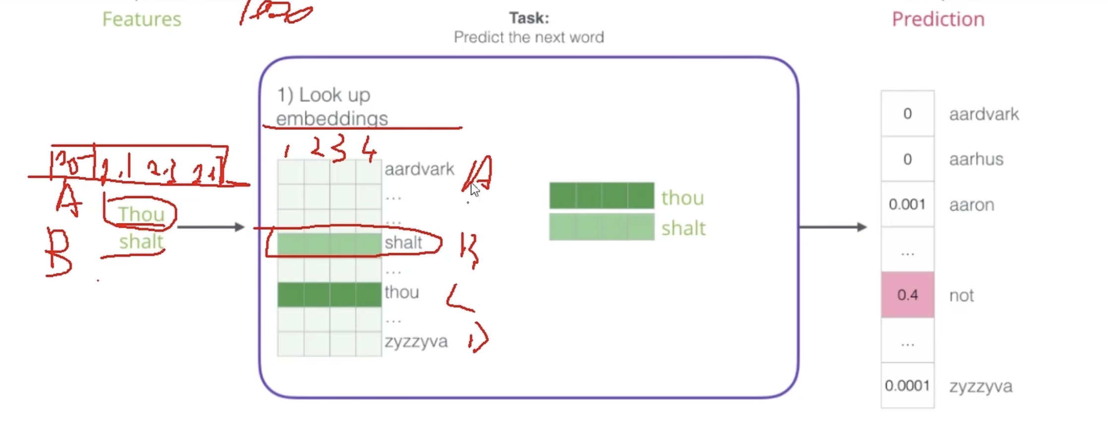
首先是查表,也就是查对应的词向量。当然这个表哪来的呢,一开始我们随机初始化所有的向量,我们知道在深度学习模型中前向传播计算Loss function,反向传播利用loss function更新权重参数,
随着训练进行,每次都会把表进行更新,使得loss更小。
我们可以这样构造数据集,如图所示:
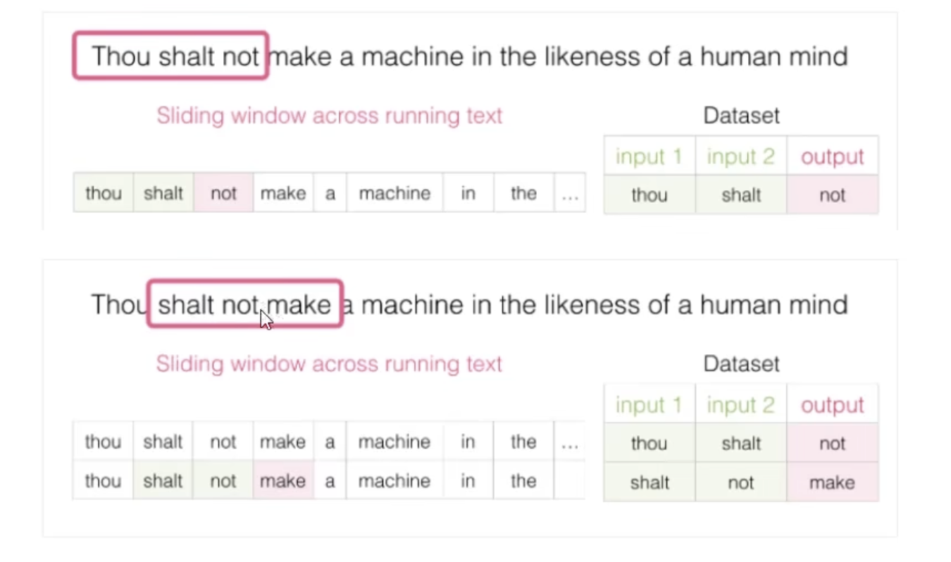
一次一次滑动形成输入输出数据集。
caffe中的prototxt文件解读
这个文件一般用来存储模型,或者说网络的架构。
架构中含有每一层网络的具体参数,参考这个链接https://blog.csdn.net/github_37973614/article/details/81810327
我们补充一个重要的东西就是im2col层,用来帮助卷积运算。
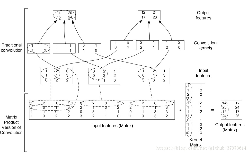
可以看到将一个图片,按照卷积核的大小来框成一个新矩阵,也就是左下角矩阵,其中每一列代表一个图片。
可以看到输入是1x3x3x3(NxCxHxW),而卷积核是2x3x2x2(NxCxHxW),所以输出肯定有两个batch,然后每一个都是卷积核大小也就是2x2,而右下角为im2col之后的输出形式,显然包含了我们所需要的输出特征,也就是两层,每一层向量长度是4。
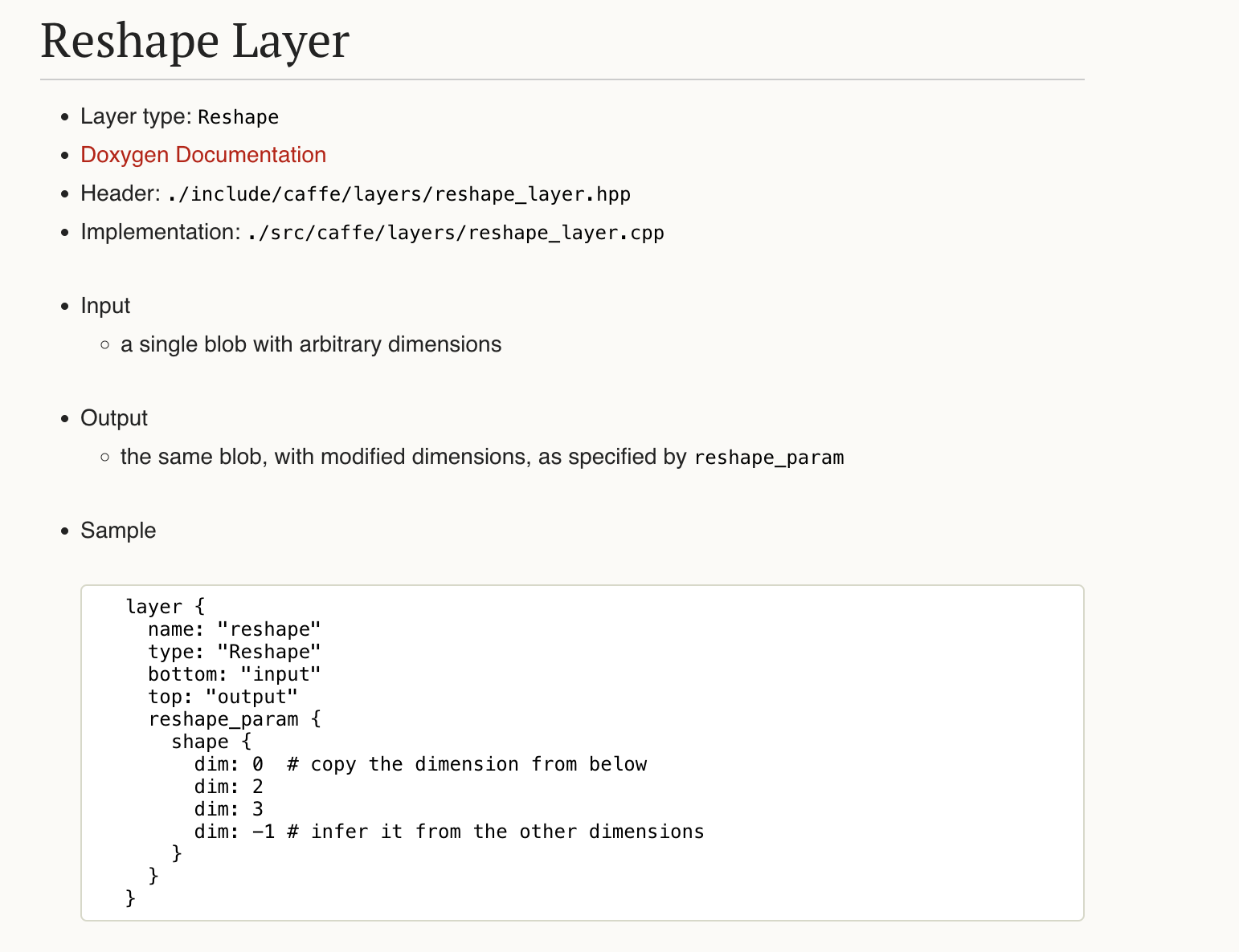
对于这个prototxt文件中的reshape层,其中,shape{}里面分别会标注第一维一直到最后一维的维数,如果是正数的话,那么正数就是维数,比如dim=2处索引是1,而索引1表示第二个维度,所以dim=2这一行就是第二个维度的维数是2。dim=0表示与bottom也就是输入层对应维度的维数相同。dim=-1就是别的都算完了,用元素总数除以其他维度乘积,算出最后维度。比如矩阵展开了一共24个元素,原来矩阵的第一维是2,其他都按照图中标注来算,那么输出矩阵的大小就应该是2x2x3x2即可。
1 | If "input" is 2D with shape 2 x 8, then the following reshape_param |
如果只有
1 | shape{ |
那么就和展开一样的,也称和展平层(flatten layer)相同。
下面是额外参数axis
1 | // axis may be non-zero to retain some portion of the beginning of the input |
对于num_axes,稍微有点难理解
1 | // num_axes specifies the extent of the reshape. |
这是表示重塑的范围,就是只有[axis, axis + num_axes]的范围才会被重塑,其余范围不变!
我们就看最后一个例子,想要表示2x1x8,最后一行中,给出了一个dim=1,但是后面给出axis=1和num_axes=0,也就是说只有[1]这个维度才会被重塑,重塑成dim=1,而[1]是第二维,所以dim=1并不是指第一维变成1,因为第一维变成1就无法实现我们想要的输出2x1x8了,只有第二维变成1,然后根据nun_axes性质,其余维度不变,最终结果大小为2x1x8。
 wechat