Matlab wireless communication foundation

QAM modulation

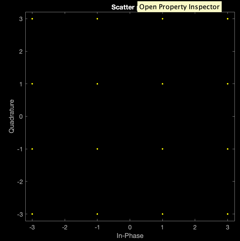
We use Matlab toolbox to realize QAM modulation easily.

1
2
3
4
5
6
7
8
srcBits = randi([0, 1], 20000, 1);%列向量,信源,而且注意16QAM是4位一组,所以2000应该为4的倍数
modOrder = 16;
modOut = qammod(srcBits, modOrder, "InputType", "bit");
scatterplot(modOut);
%画出星座图
demodOut = qamdemod(chanOut, modOrder, "OutputType", "bit");
check = isequal(srcBits, demodOut);
disp(check);

Here is the QAM graph.

image-20230910003431995

QAM modulation and AWGN(Additive White Gauss Noise)channel

脚本如下

1
2
3
4
5
6
7
8
9
10
11
12
13
14
15
16
17
18
19
srcBits = randi([0, 1], 20000, 1);%设置信源
modOrder = 16;%设置调制电平等级,也就是4bits.

snr1 = 1.5;%设置一个糟糕的信噪比,当然,后面为了实验,我们会改动信噪比。
modOut1 = qammod(srcBits, modOrder, "InputType","bit", "UnitAveragePower",true);%进行qam调制
%注意这里我们设置调制信号的平均功率为1
chanOut1 = awgn(modOut1, snr1);%通过awgn信道。
scatterplot(chanOut1);%画出散点图
demodOut1 = qamdemod(chanOut1, modOrder, "OutputType", "bit", "UnitAveragePower", true);%进行解调
check = isequal(srcBits, demodOut1);%检查信源和收到的解调信号是否相同。
disp(check);

snr2 = 20;%看信噪比为20时的正确率
modOut2 = qammod(srcBits, modOrder, "InputType", "bit", "UnitAveragePower", true);
chanOut2 = awgn(modOut2, snr2);
scatterplot(chanOut2);
demodOut2 = qamdemod(chanOut2, modOrder, "OutputType", "bit", "UnitAveragePower", true);
check = isequal(srcBits, chanOut2);
disp(check);

Calculate Bit Error Rate(BER)

1
2
3
4
5
6
7
8
9
10
11
12
13
14
15
16
17
numBits = 20000;
modOrder = 16;%the same parameters
%Create source signal
srcBits= randi([0, 1], numBits, 1);
modOut = qammod(srcBits, modOrder, "InputType", "bit", "UnitAveragePower", true);

%Apply AWGN
SNR = 10; %dB
chanOut = awgn(modOut, SNR);
scatterplot(chanOut);%draw the scatter graph of passing AWGN

demodOut = qamdemod(chanOut, modOrder, "OutputType", "bit", "UnitAveragePower", true);
isBitError = srcBits ~= demodOut;%Now we compare the source bits and the bits from %demodulation.
%Output a array, 0 represents the two bits of srcBits and demodOut are the same, vice versa.
numBitError = nnz(isBitError);
%calculate the number of 1
disp(BER);

image-20230910003223366

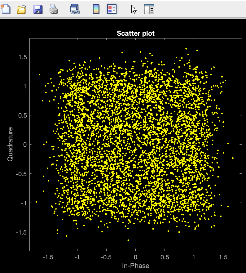
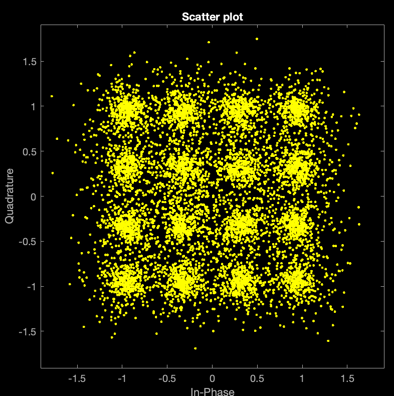
Obviously, if we add the AWGN channel, then the BER is very large, and we have to improve our SNR to cancel it.

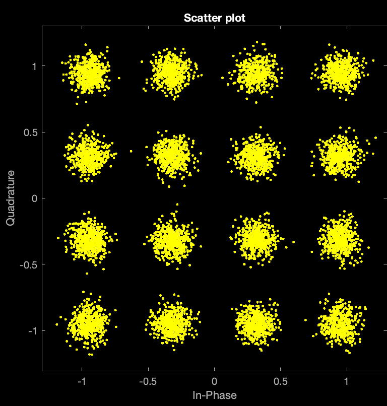
When we change BER into 20dB, let’s see the graph.

image-20230910003344406

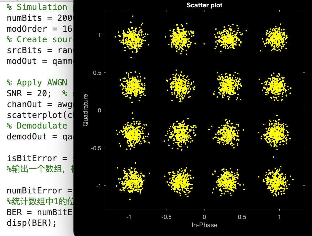
The bit can be distinguished now!
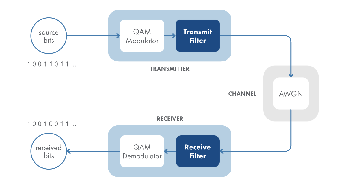
Matched Filter

image-20230910180157139

All wireless communication signals must occupy a designated frequency band, much like how vehicles occupy a lane in a highway. If the signal’s energy extend beyond that band, it interferes the signals have the frequencies that be above or below your signal.

A transmitter filter makes sure that your transmitted signal stays within its designated band.

On the other hand, the receiver also filters its input signal. Here, the filter will reduce the noise power that the downstream processing must handle.

image-20230910184047636

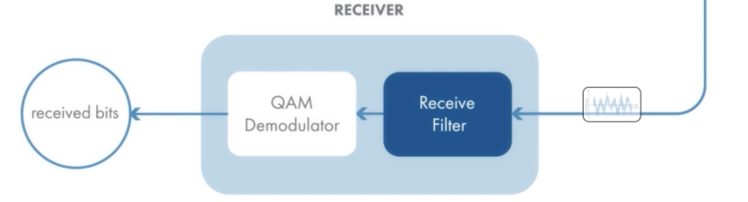
Since both transmitter and receiver filter the signals, it’s important that the two filters have matching frequency responses. These matched filters provide optimum performance in the presence of noise, because they maximize the signal to noise ratio of the output.

image-20230910184400751

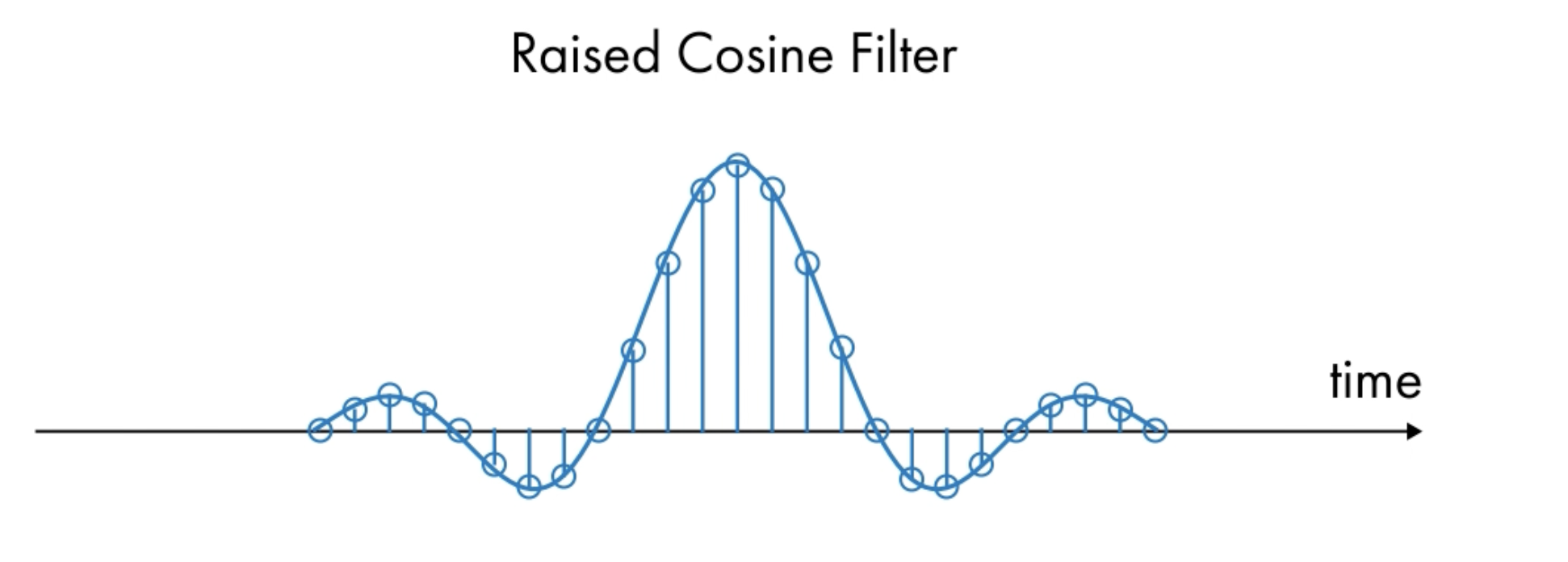
There are many types of matched filters to choose from, we use commomly used Raised Cosine Filter, because it elimates inner-symbol interference that filtering can introduce.

Reason: In the time domain, when you filter, the filter’s inpulse response can smear one symbol into the next, which can distort it!

image-20230910184718412

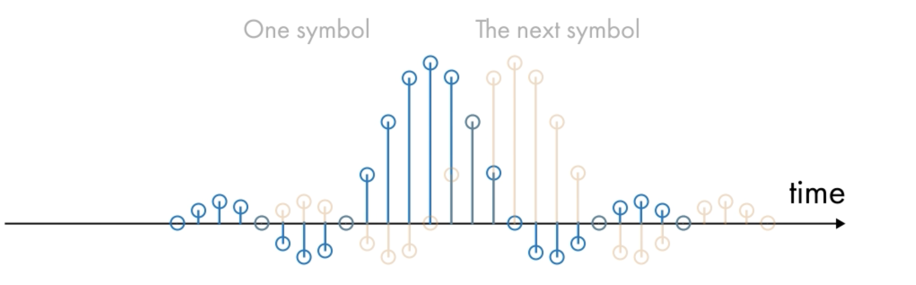
A Raised Cosine Impulse Response has a convenient property, the peak of one filter’s symbol occurs the zero crossings(其他波在此处0值) of the filter’s symbols that come before and after it.
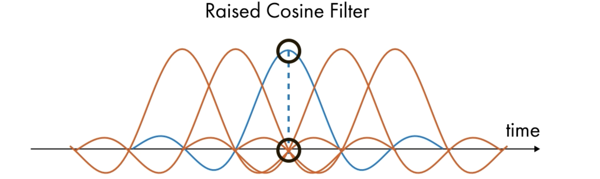
image-20230910184823109

image-20230910185036367

So!Zero ISI!

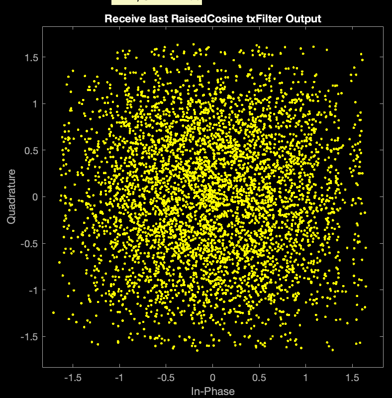
For implementation, since you need two filters, its convenient for their composite response to be the raised Cosined Filter response, so then use a Square Root Raised Cosine Filter for each,

image-20230910185352296

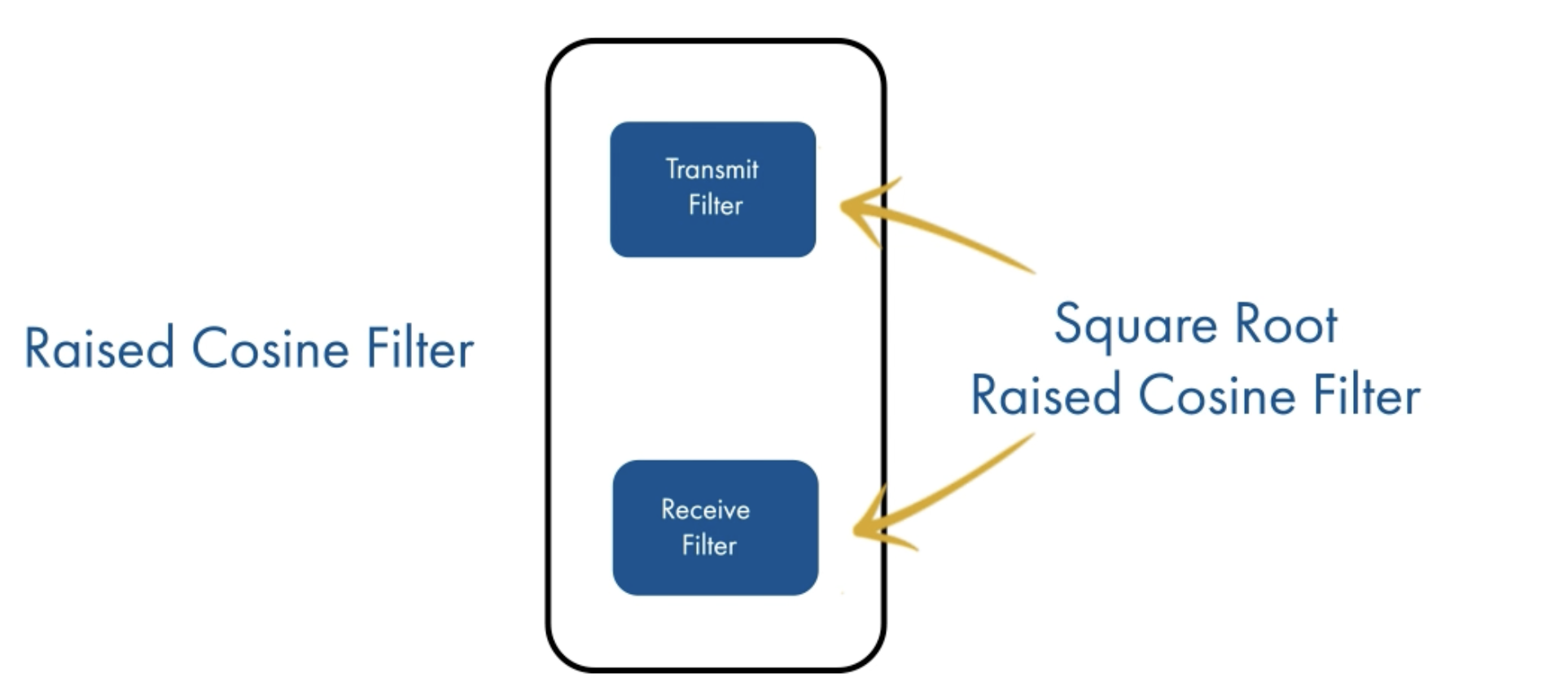
and there you have it!

image-20230910185422435

Band limited on the front end, noise reduction on the backend, and zero ISI with the composite Raised Cosine Filter.

1
2
3
4
5
6
7
8
9
10
11
12
13
14
15
16
17
18
19
20
21
22
23
24
25
numBits = 20000;
modOrder = 16;
srcBits = randi([0, 1], numBits, 1);
modOut = qammod(srcBits, modOrder, "InputType", "bit", "UnitAveragePower",true);
%匹配滤波器我们用raisedcosinefilter,形状和sample函数差不多,我们将其拆成两个部分,
%输入滤波器和输出滤波器,所以每个部分用其方根即可!
%下面这个就已经是方根!
txFilt = comm.RaisedCosineTransmitFilter;
rxFilt = comm.RaisedCosineReceiveFilter;%
txFiltOut = txFilt(modOut);

SNR = 7;
chanOut = awgn(txFiltOut, SNR, "measured");
%measured调整信号功率,因为经过了滤波器。
rxFiltOut = rxFilt(chanOut);

if exist("rxFiltOut", "var")
scatterplot(rxFiltOut);
demodOut = qamdemod(rxFiltOut, modOrder, "OutputType", "bit", "UnitAveragePower", true);

end
%下面创建一个功率谱分析仪,查看发射滤波器输出和AWGN信道输出的功率谱,无噪声信号为黄色,
%加AWGN噪声的信号为蓝色。
specAn = dsp.SpectrumAnalyzer("NumInputPorts", 2, "SpectralAverages", 50, "ShowLegend", true);
specAn(txFiltOut, chanOut);

Mathpath signal recession

In wireless communications, the transmitted signal generally has reflected off many different surfaces before reaches the receiver.

image-20230910190031442

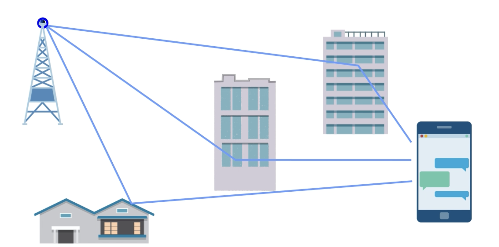
These reflections resolve a phenomenon called multipath. Multipath basically means the transmitted signal has travelled a multiple different path by the time it reaches the receiver.

image-20230910190234525

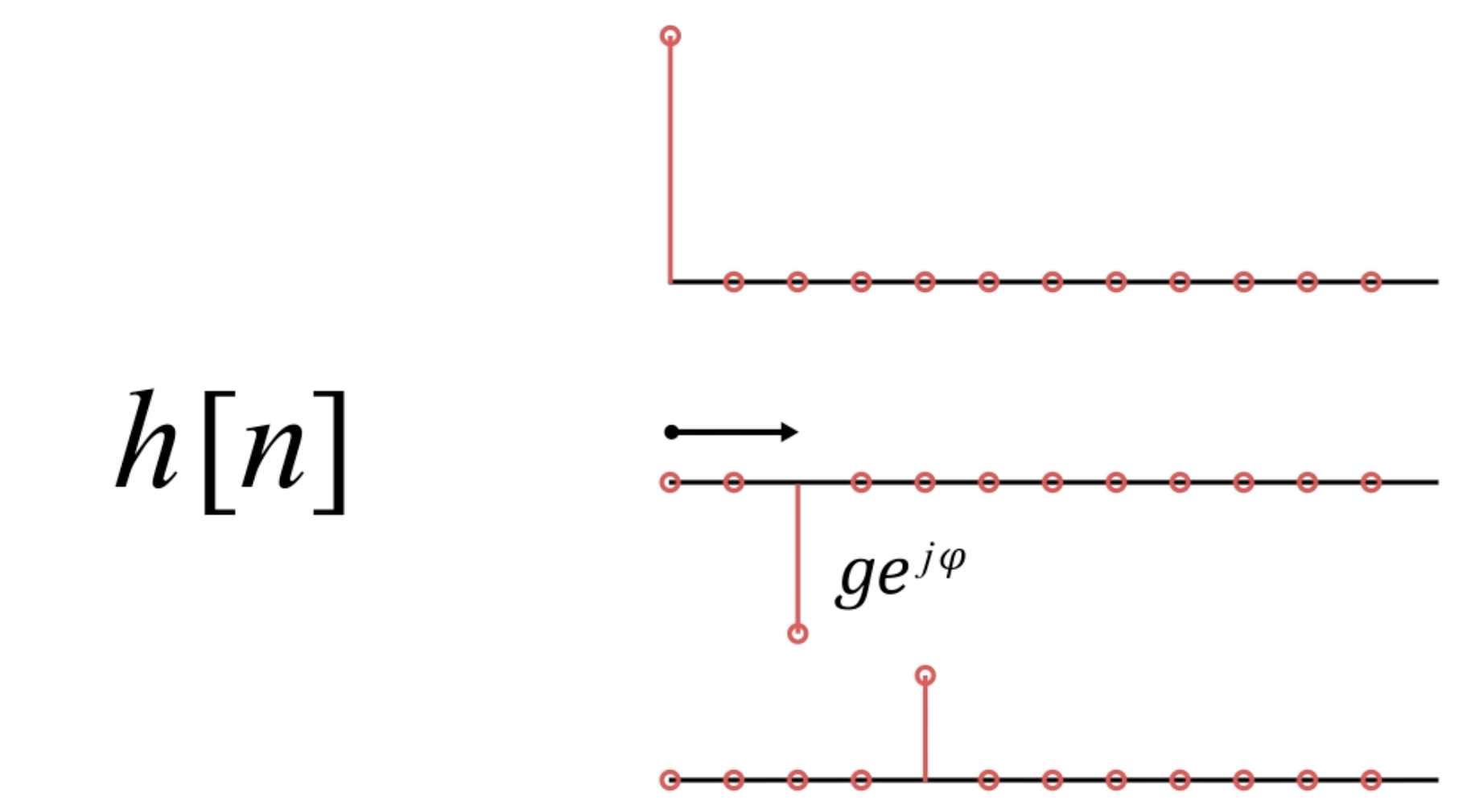
Each path changes the signal while it’s on its way. For example, it could have a different gain or take longer to arrive.

image-20230910190418709

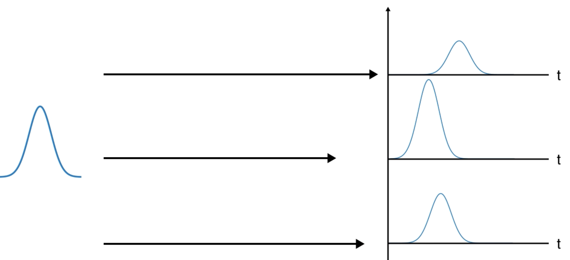
As a result, the receiver gets multiple superimposed copies.And sees a time smear version of a transmitted signal.

image-20230910190602544

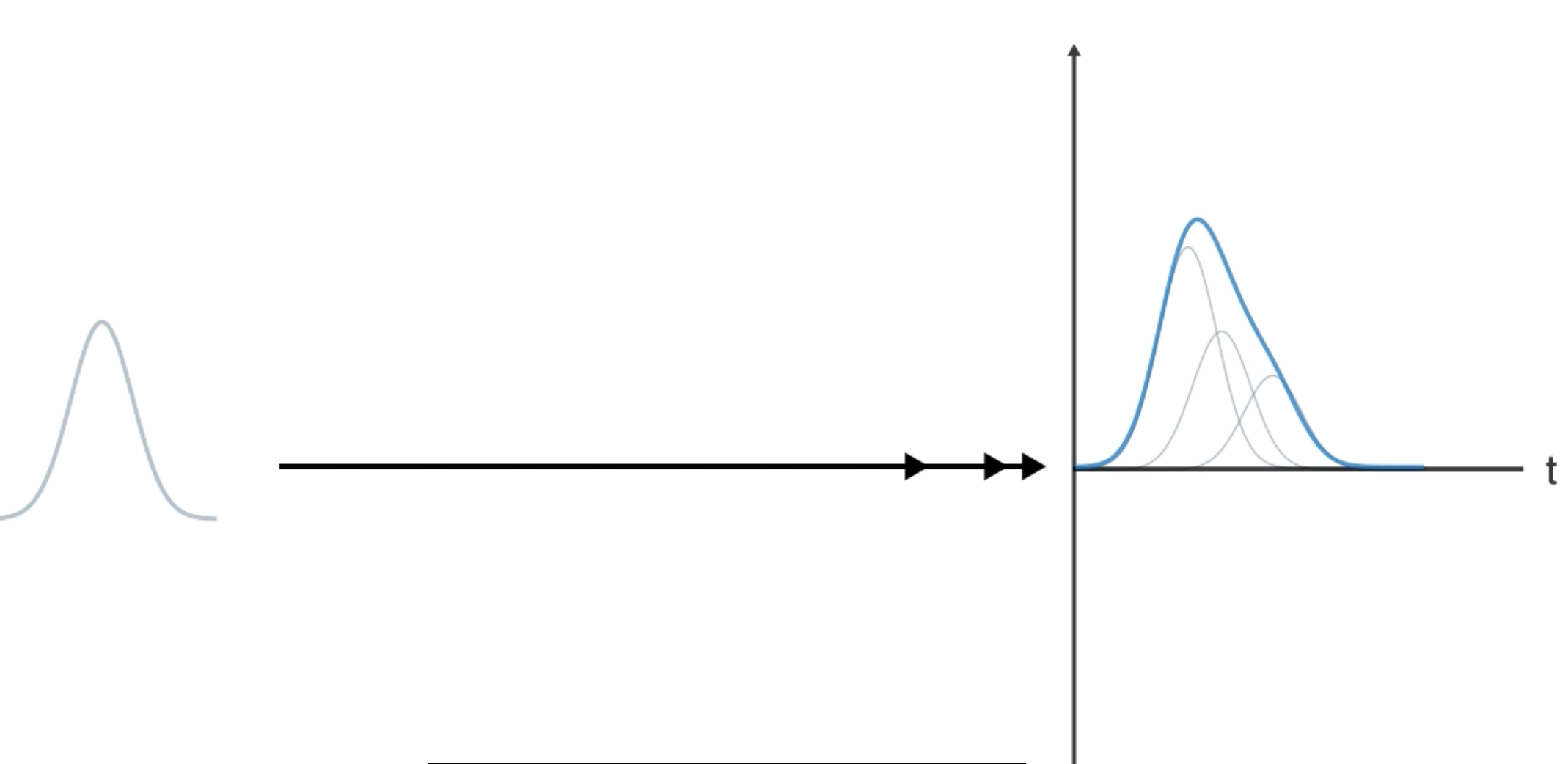
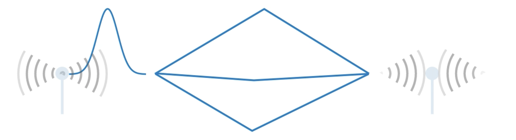
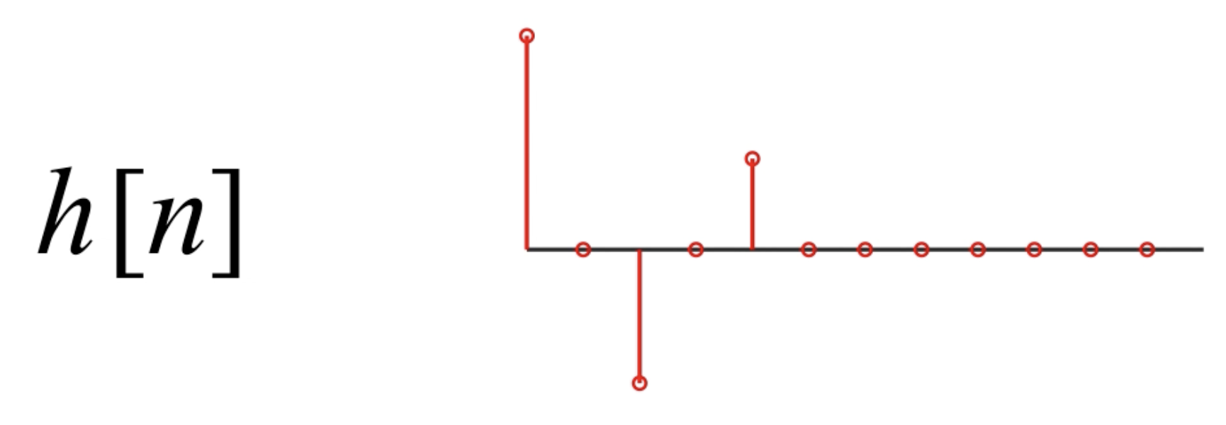
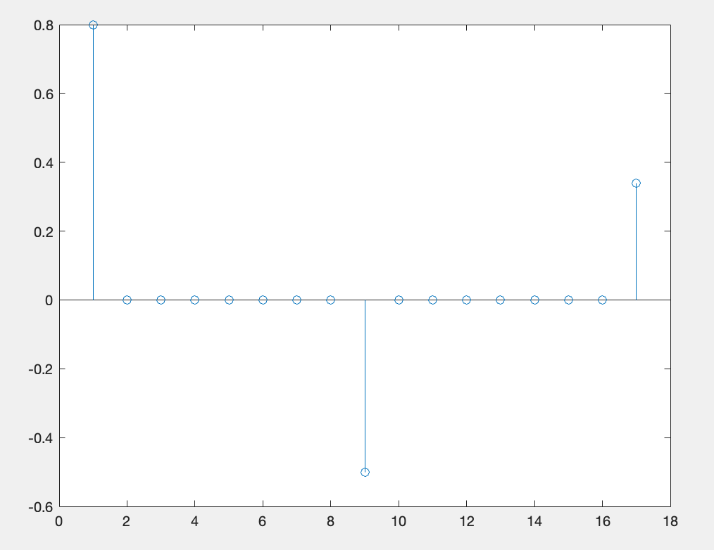
Mathematically, it’s simply the sum of the impulse responses for the various path, including the time delay and gain and phase change for each path.

image-20230910190848353

image-20230910190911026

1
2
3
4
5
6
7
8
9
10
11
12
13
14
15
16
17
18
19
20
21
22
23
24
25
26
27
28
29
30
31
32
33
34
35
36
37
38
39
40
41
42
43
44
45
46
47
48
49
50
51
52
53
54
55
56
57
58
59
60
61
62
%Single Carrier Link with Multipath Channel
numBits = 20000;
modOrder = 16;
bitsPerSymbol = log2(modOrder);
%每个符号有4位
txFilt = comm.RaisedCosineTransmitFilter;
rxFilt = comm.RaisedCosineReceiveFilter;
srcBits = randi([0, 1], numBits, 1);
modOut = qammod(srcBits, modOrder, "InputType", "bit", "UnitAveragePower", true);
%完成基本调制

%多径信道相当于FIR滤波器,也就是多个离散时间点上的冲击响应的和,也就是相当于信号卷积
%上一个sinc函数,sinc上每个离散时间点的值相当于一条径,并且多径我们认为它是有限条路径。
%而FIR滤波器在matlab中可以用列向量来表示。
txFiltOut = txFilt(modOut);

spacing = zeros(1, 7);
mpChan = [0.8, spacing, -0.5, spacing, 0.34].';
%或者是spacing = zeros[7, 1];mpChan = [0.8; spacing; -0.5; spacing; 0.34];
%也可以表示列向量
disp(mpChan);
stem(mpChan);%这就相当于多径信道的冲激响应

mpChanOut = filter(mpChan, 1, txFiltOut);
%这里是过滤波器,把mpChan看成滤波器,进行卷积运算,FIR滤波器的分母是1,这是显然的
%最后一个参数表示对txFiltOut操作

%先经过多径!再经过awgn信道!牢记
if exist("mpChanOut", "var")
SNR = 15;
chanOut = awgn(mpChanOut, SNR, "measured");
rxFiltOut = rxFilt(chanOut);
scatterplot(rxFiltOut);
title("Receive last RaisedCosine txFilter Output");
demodOut = qamdemod(rxFiltOut, modOrder, "OutputType", "bit", "UnitAveragePower", true);

%calculate the BER

delayInSymbols = txFilt.FilterSpanInSymbols / 2 + rxFilt.FilterSpanInSymbols / 2;
%我们要比较位,所以要确定延迟的位数,而不是符号数,16QAM4个位一个符号是四维信号
delayInBits = delayInSymbols * bitsPerSymbol;

srcAligned = srcBits(1:(end - delayInBits));
%提取除最后的delayInBits之外的所有位!从源序列中获取对其位。
%end代表最后一位的索引,
demodAligned = demodOut((delayInBits + 1):end);%接受序列中,delayInBits在最前面几位
%提取,并且获得对齐位。

%最后计算误码率
numBitErrors = nnz(demodAligned ~= srcAligned);
numAlignedBits = length(srcAligned);
BER = numBitErrors / numAlignedBits;
disp(BER);
end

%查看发射信号的频谱和信道输出。发射信号为黄色,而含噪多径信号为蓝色。
%接收到的信号的频谱的通带中有一个"缺口”,这会使单载波波形发生显著扭曲。这种现象称为频率选择性多径,因为信道衰减或增益的水平取决于频率。
%下面利用频谱分析仪查看频率选择性衰落!
specAn = dsp.SpectrumAnalyzer("NumInputPorts", 2, "SpectralAverages", 50, "ShowLegend", true);
specAn(txFiltOut, chanOut)
%chanOut相当于经过多径和awgn的共同作用之后的结果。
%txFiltOut只是刚刚经过匹配滤波器确保无码间干扰的结果

image-20230910191131840

image-20230910191111978

image-20230910191158729

OFDM(Orthogonal Frequency Division Multiplexing)

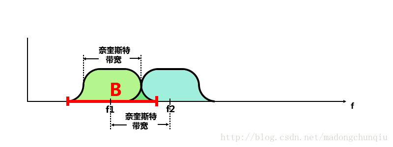
The multiple carriers are used to tramsmit data, each carrier has different frequency, in OFDM, according to Nyquist Bandwidth, the bandwidth efficiency has been improved and it can guarantee no inter-symbol interference(ISI)!
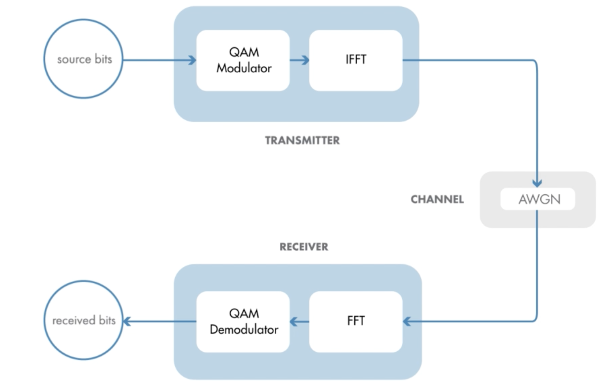
img

1
2
3
4
5
6
7
8
9
10
11
12
13
14
15
16
17
18
19
20
21
22
23
24
%This is a simple OFDM system, using IFFT as a modulator, FFT as a demodulator.
numBits = 32768;%because this is a power of 2.
modOrder = 16;
srcBits = randi([0, 1], numBits, 1);
qamModout = qammod(srcBits, modOrder, "InputType", "bit", "UnitAveragePower", true);
scatterplot(qamModOut);%draw a basic QAM constellation.

%passing OFDM
ofdmModOut = ifft(qamModOut);%It is equal to add OFDM in the source.
if exist("ofdmModOut", "var")
SNR = 20;
chanOut = awgn(ofdmModOut, SNR, "measured");%transmit OFDM data adding AWGN
end

ofdmDemodOut = fft(chanOut);
scatterplot(ofdmDemodOut);%draw the scatter diagram

if exist("ofdmDemodOut", "var")
qamDemodOut = qamdemod(chanOut, modOrder, "OutputType", "bit", "UnitAveragePower", true);
numBitErrors = nnz(srcBits ~= qamDemodOut);%calculate Bits Error Rate
BER = numBitErrors / numBits;
end

%we can adjust SNR(dB)

image-20230910015043144

This is the OFDM-demodulated signal.

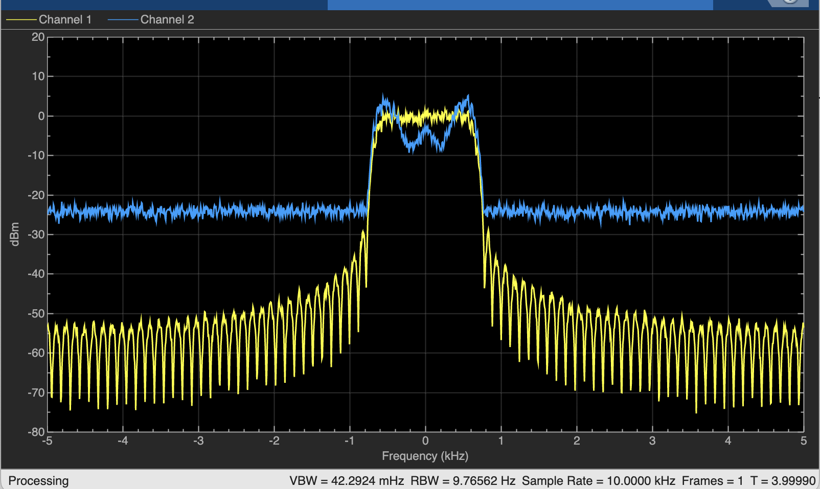
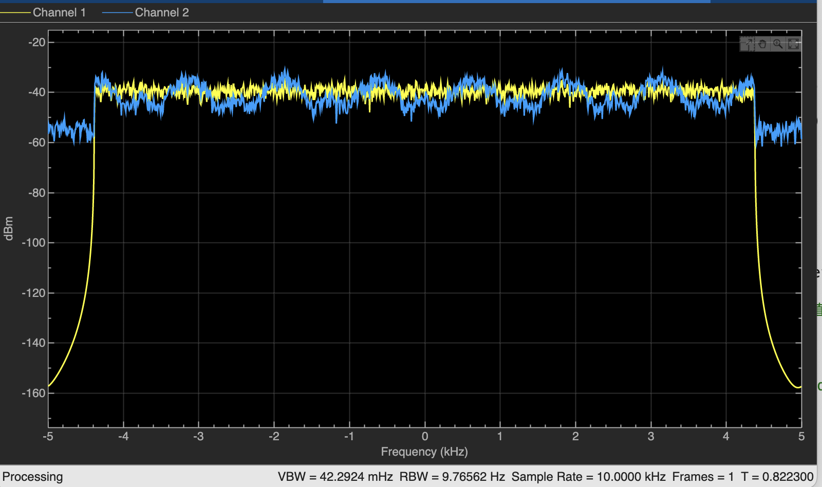
Let’s see the frequency-magnitude graph of OFDM.

image-20230910110545602

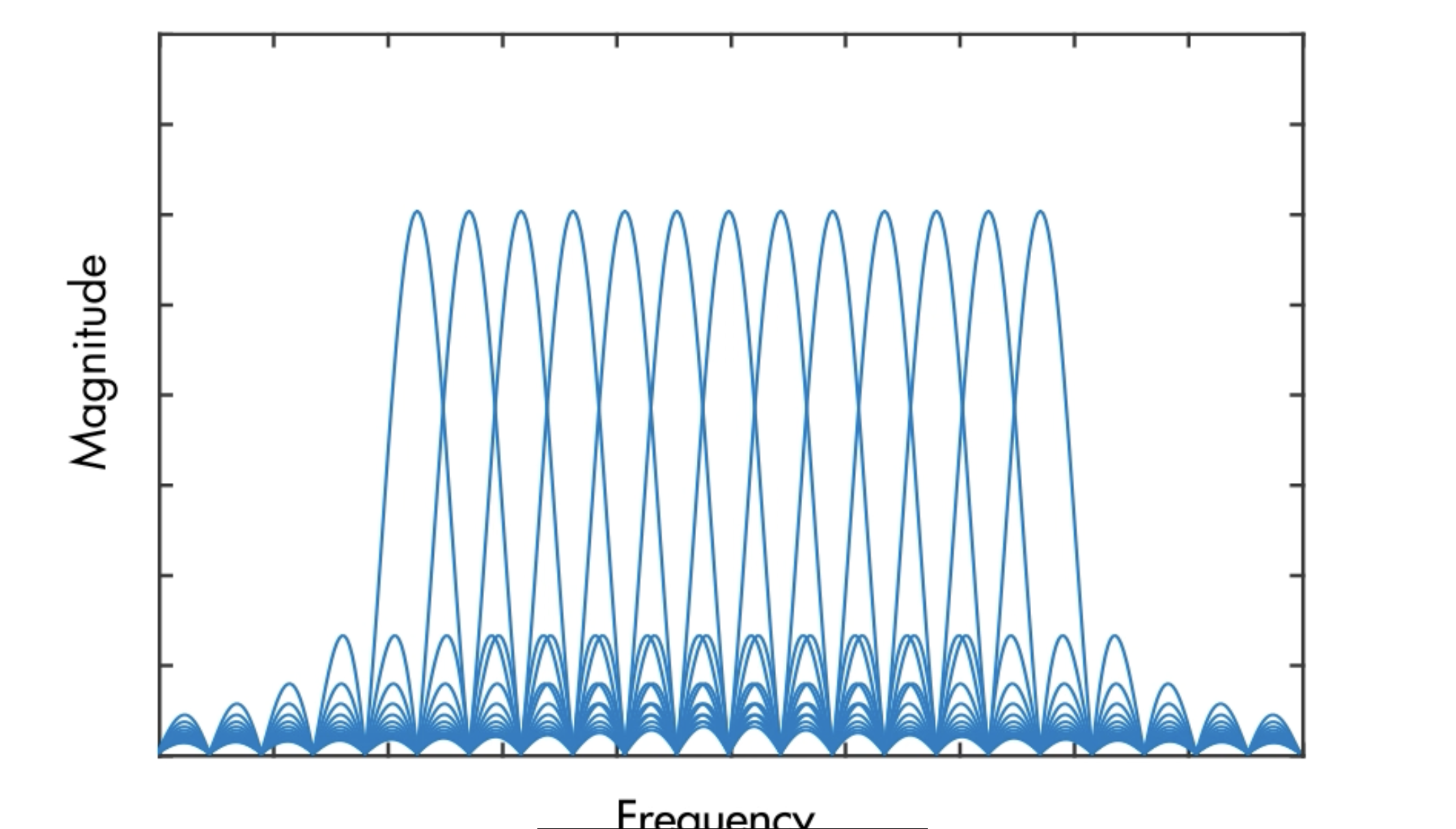
So what makes orthogonality in OFDM? Let’s zoom in to find the answer.

image-20230910110638698

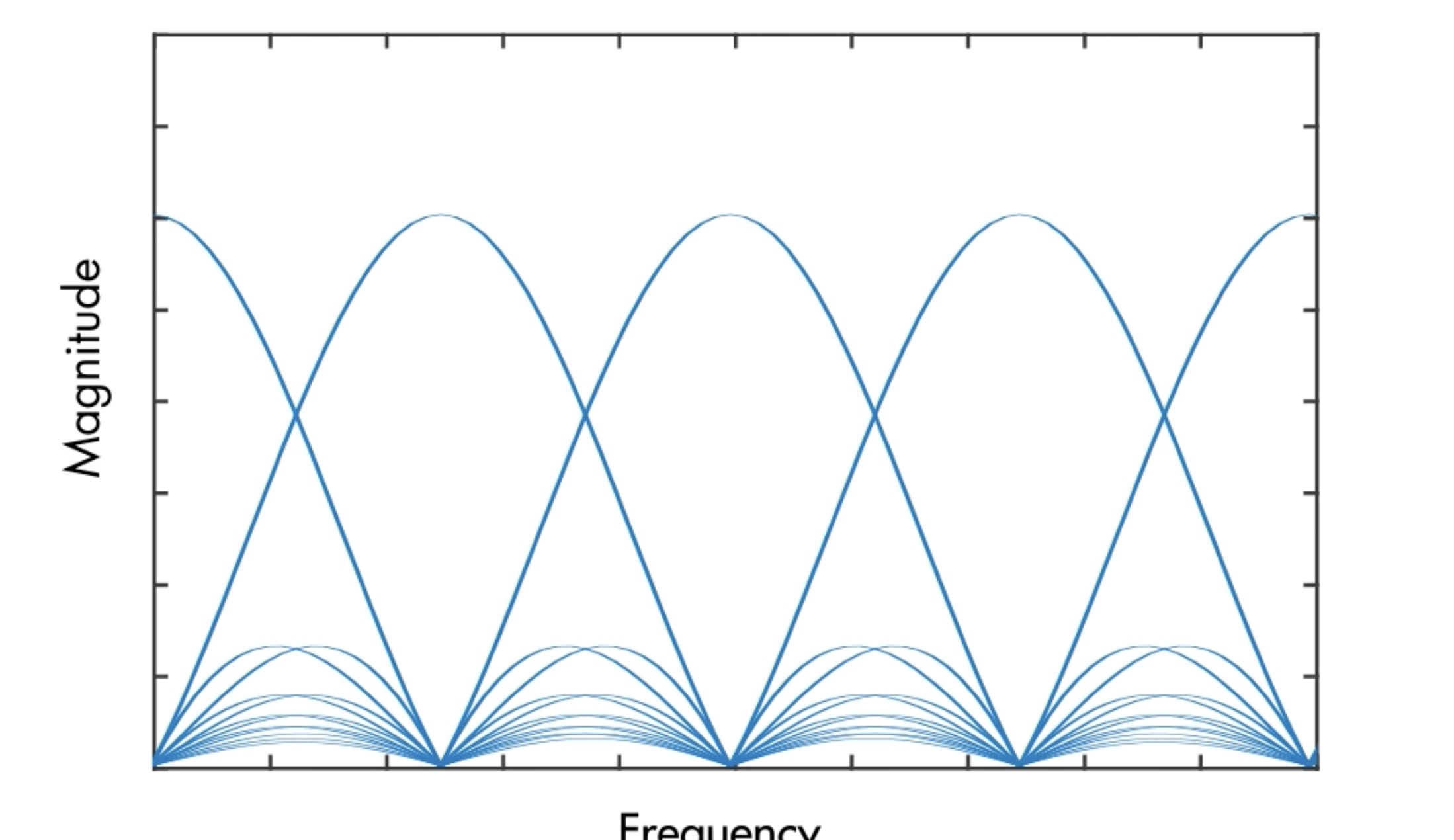
The peak of each carrier is precisely at the zero crossing of all the others, which means none of the sub-carriers interfere with each others.

And each carrier with $a_m$ as the cofficient, so the addition of the carriers can be

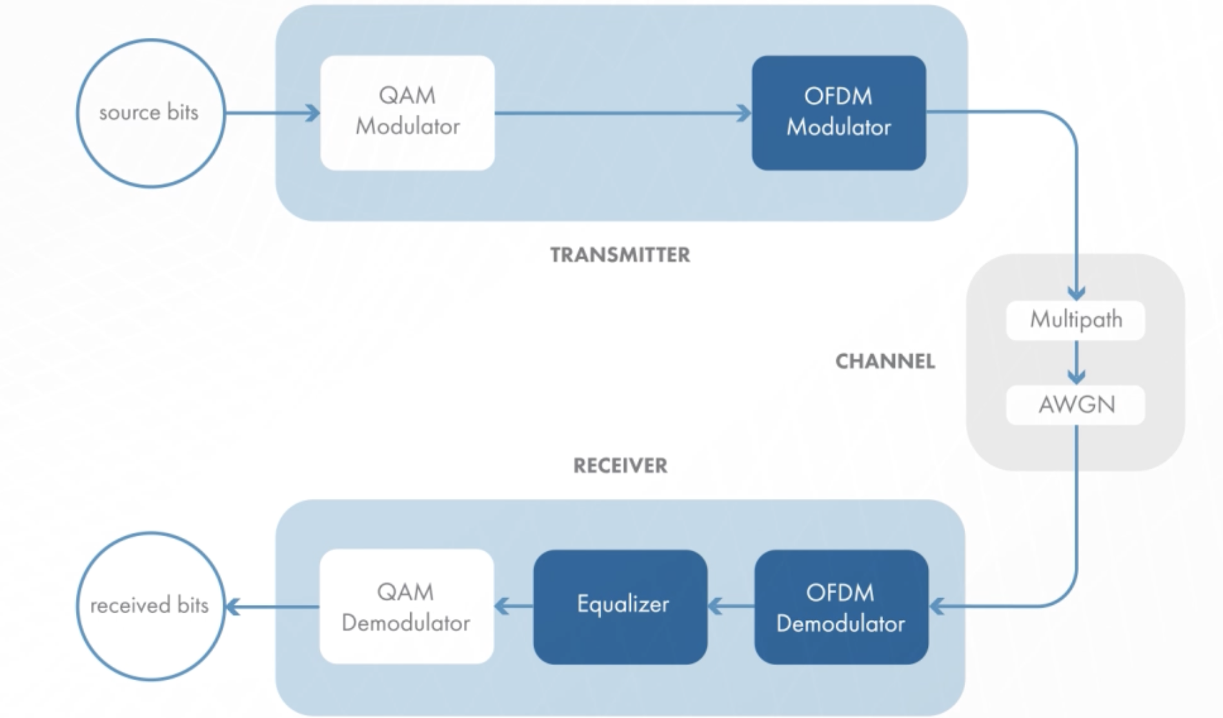
In fact it is a IDFT, which can be efficiently implemented with the IFFT! So the simplest possible OFDM link uses the IFFT in the transmitter, followed by the FFT in the receiver!

image-20230910111333748

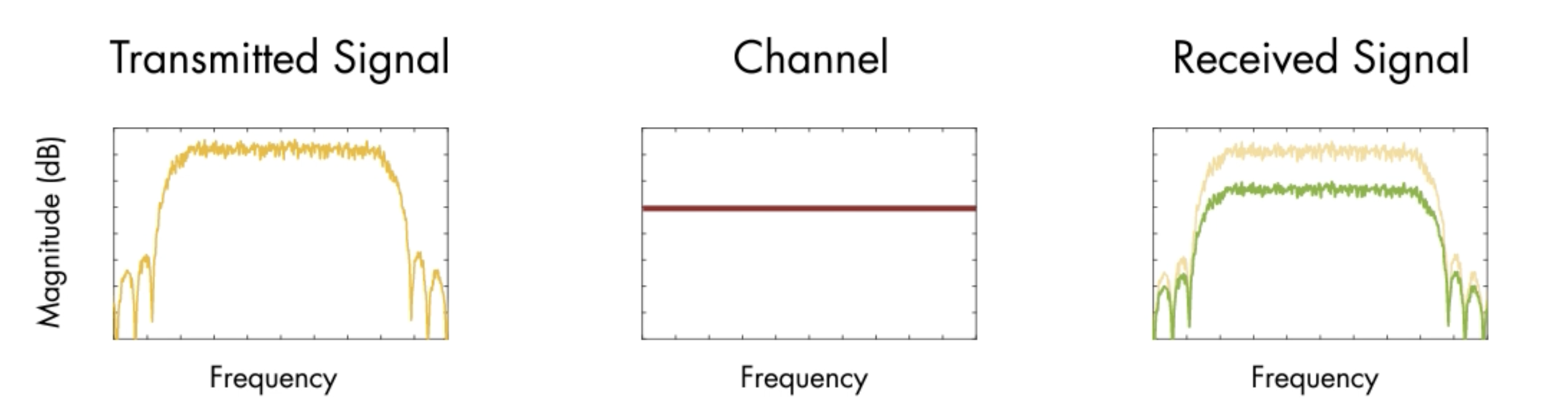
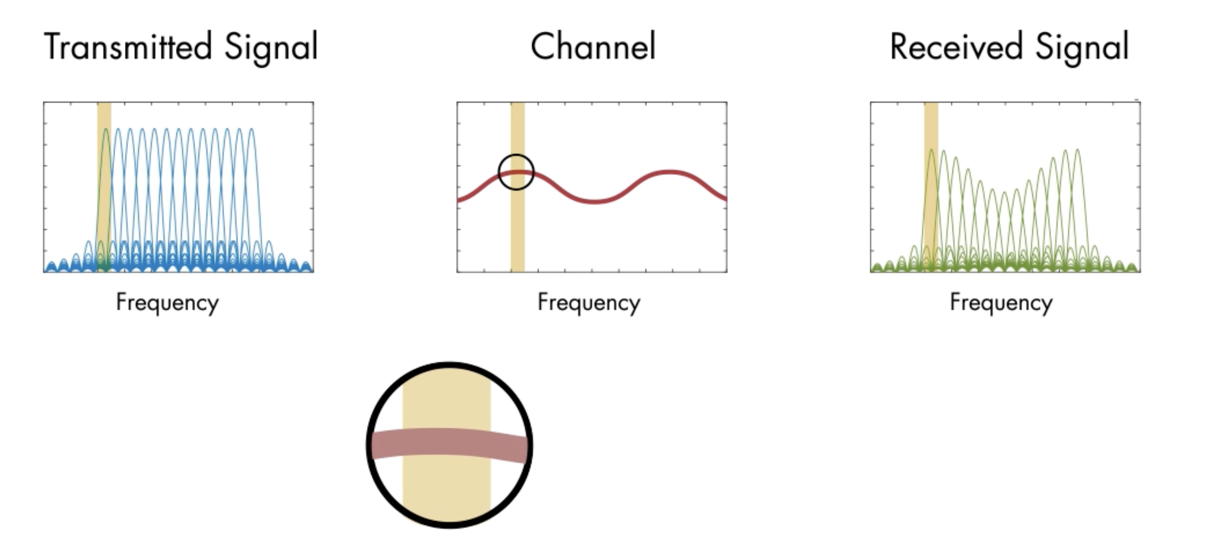
But it doesn’t actually help much with the multipath channel. A channel is basically a filter, ideally, that filter will be spectrally flat across the bandwidth of the signal.

image-20230910111719043

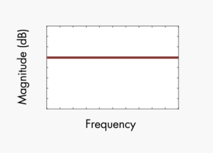
Then you can compensate for the channel signal loss and phase change with the simple complex gain in the receiver.

image-20230910111945501

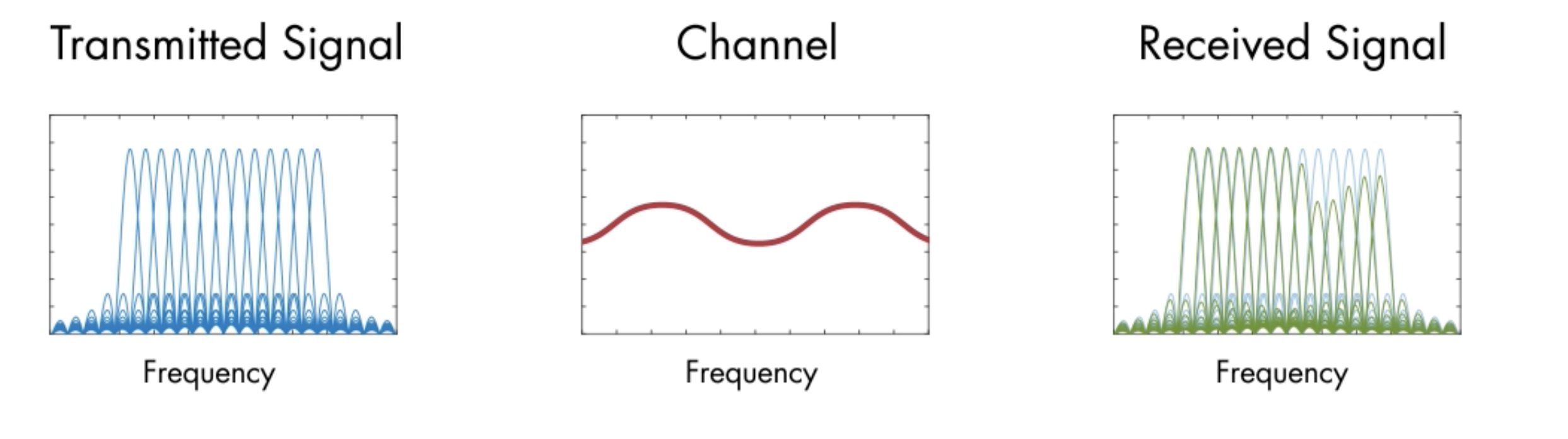
But a multipath channel spectrum can vary across the signal’s bandwidth, this causes the frequency selected fading(频率选择性衰落), where different frequencies fade different amounts.

image-20230910112413638

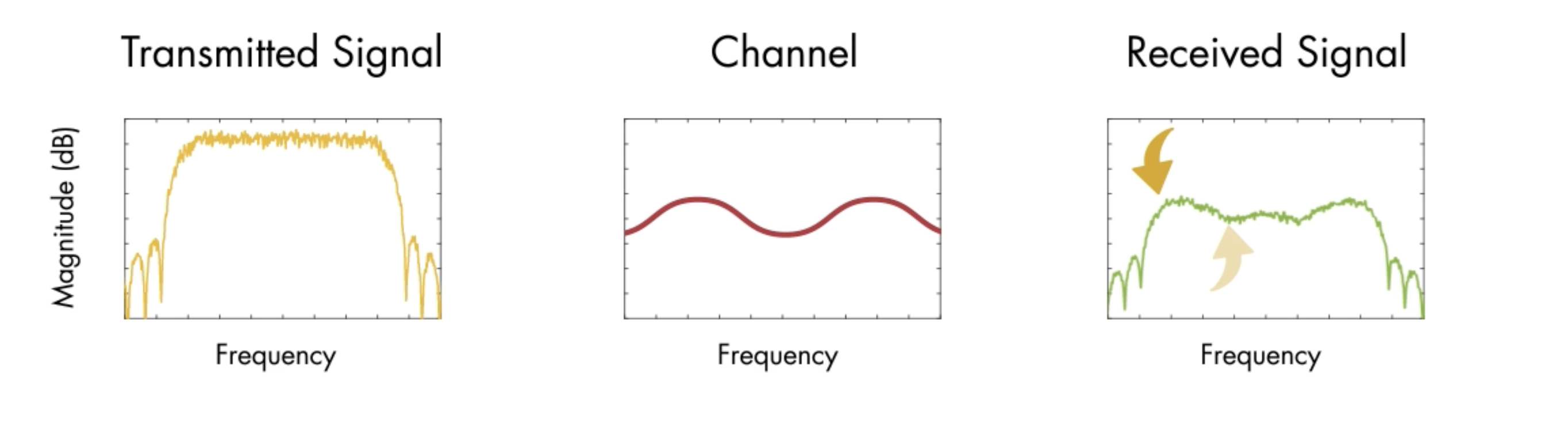
The receiver needs an equalizer to remove all the peaks and valleys created by the channel.

image-20230910112550506

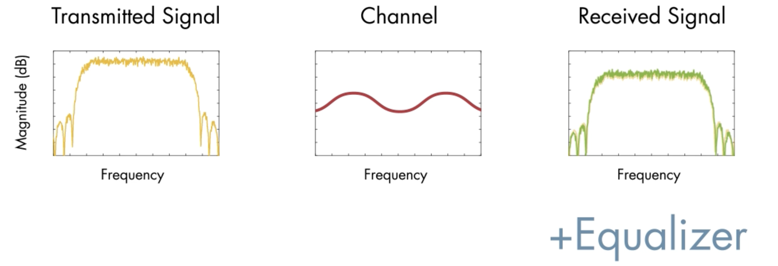
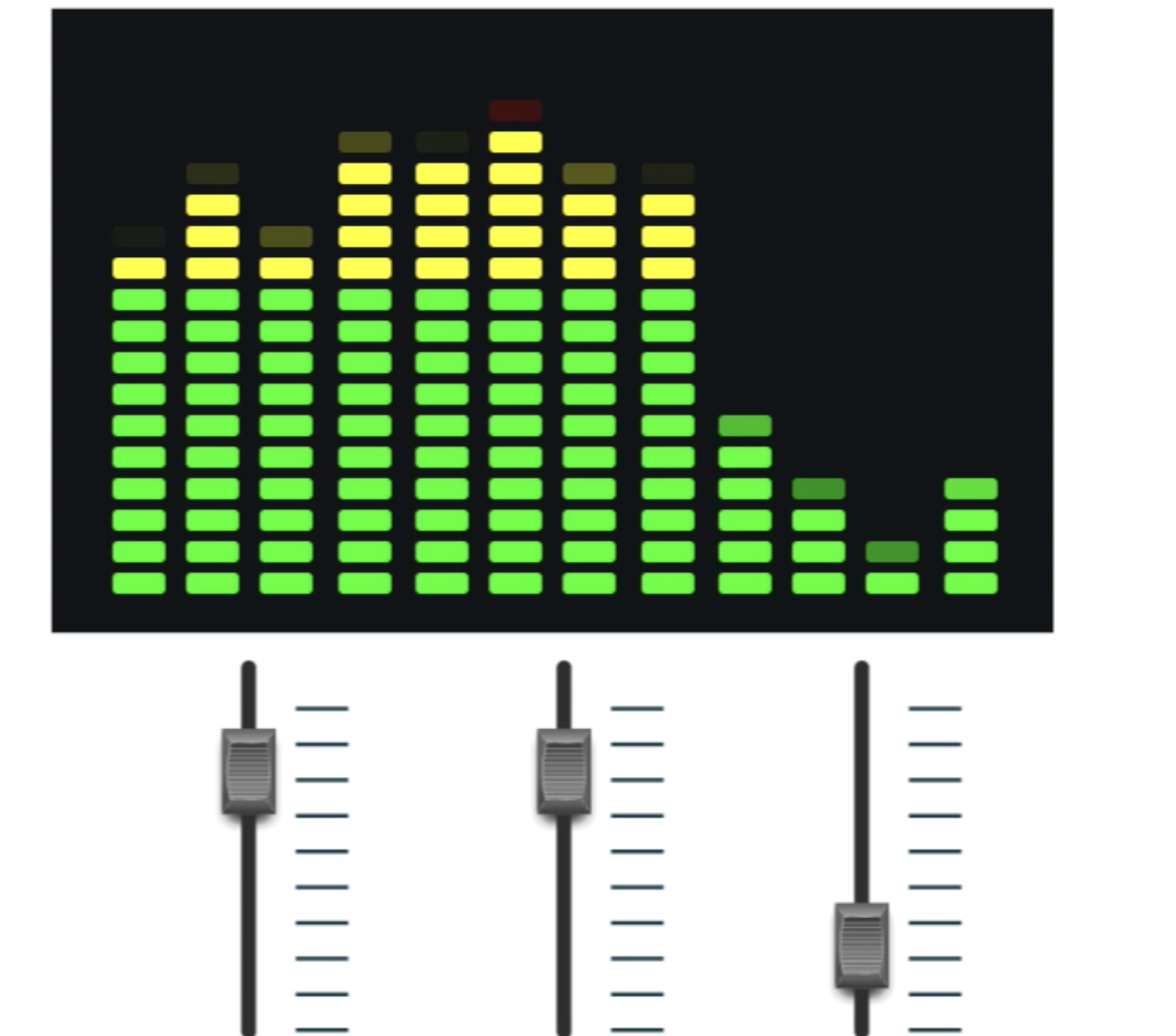
The secret of the OFDM receiver is that how it performs the equalization. It can increase of decrease the gain of different frequency, to create the best listening experience!

image-20230910112719297

OFDM turns the high rates signal into parallel low rates signals. Each low-rate signal has a narrow bandwidth. So it encounters a channel whose spectra is relatively flat!

image-20230910113053700

That means the equalizer can simply apply a complex gain, and to each sub-carrier seperately , removing the peaks and valleys.

image-20230910113247685

And since this equalization happens in the frequency domain, implementation is easy!

image-20230910152131665

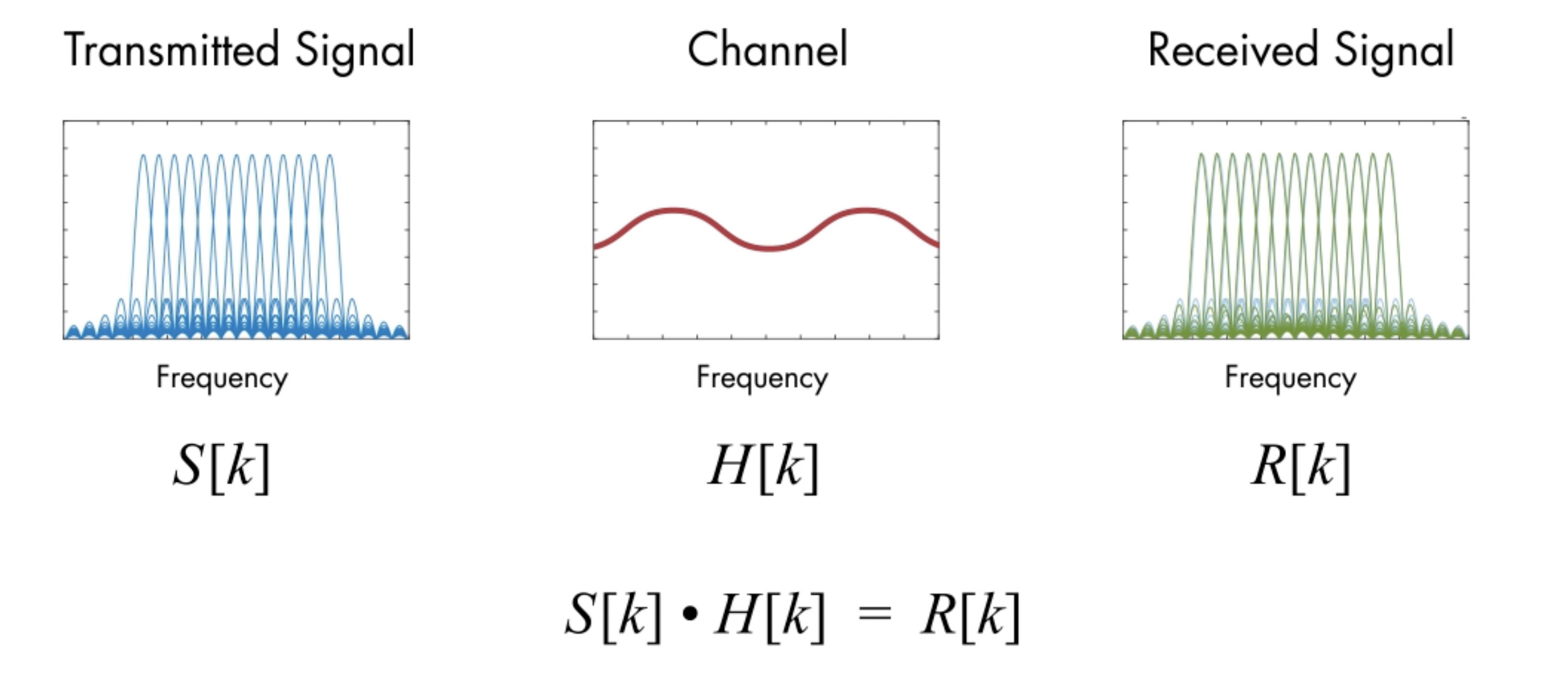
You can estimate the channel, then simply divide to get the estimate of the transmitted signal.

There is one defect of this approach. The equation above only holds if the channel performs a circular convolution on the signal.

However the reality is the channel performs a linear convolution, because it is just a filter.

If the signal is periodic, linear convolution and circular convolution are the same!

Then let’s simply make our signal periodic!

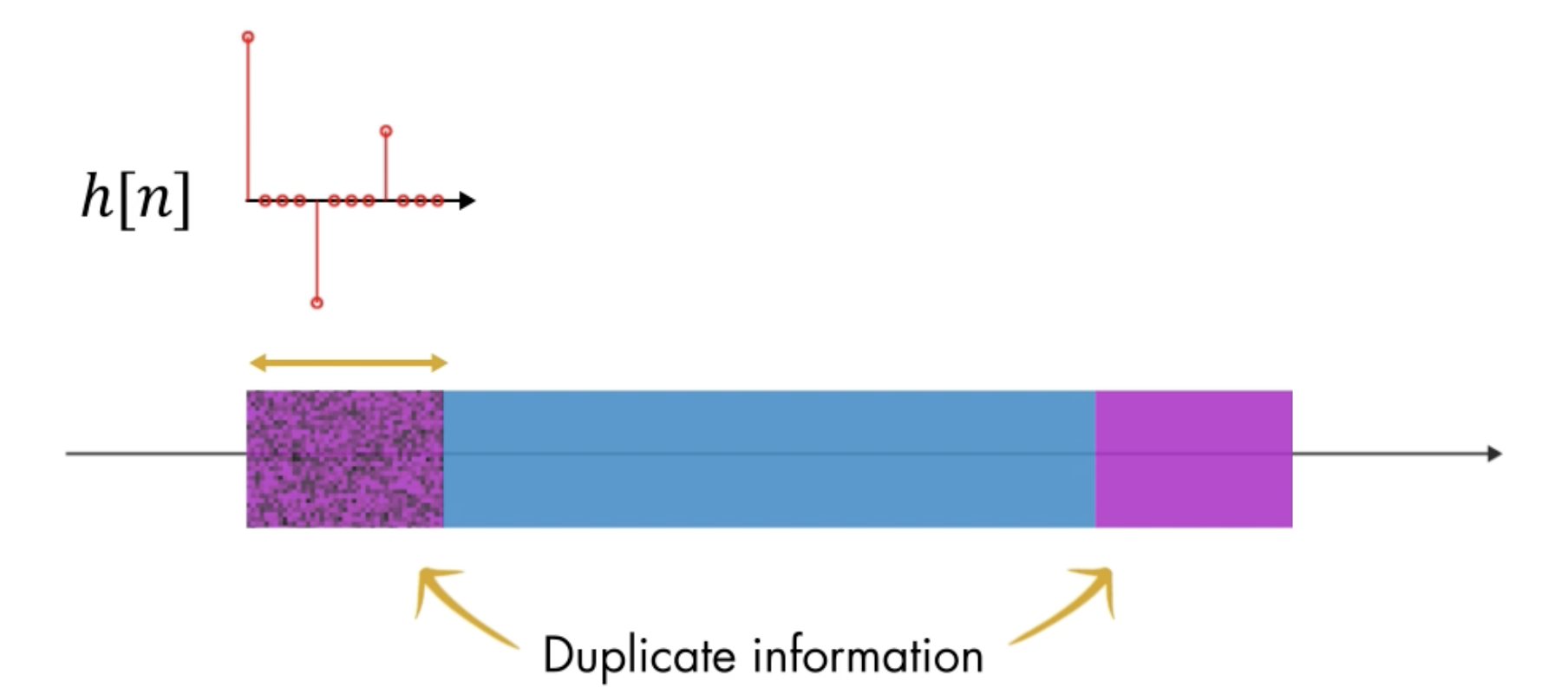
Take an OFDM symbol, take some time domain sample from the end, and then prepend them to the beginning.

image-20230910153157123

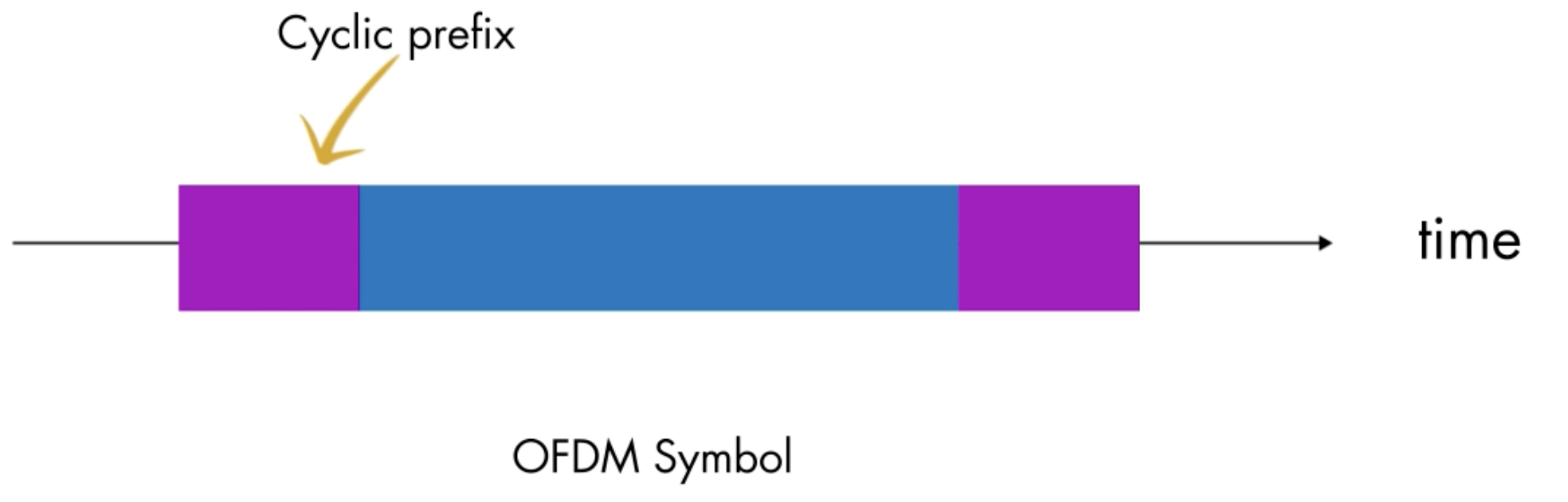
It is important that the cyclic prefix is at least as long as the channel inpulse response. The cyclic prefix will get impacted by the time smearing and the multipath channel. Since it’s duplicate information, it doesn’t really matter if it gets corrupted.

image-20230910153523980

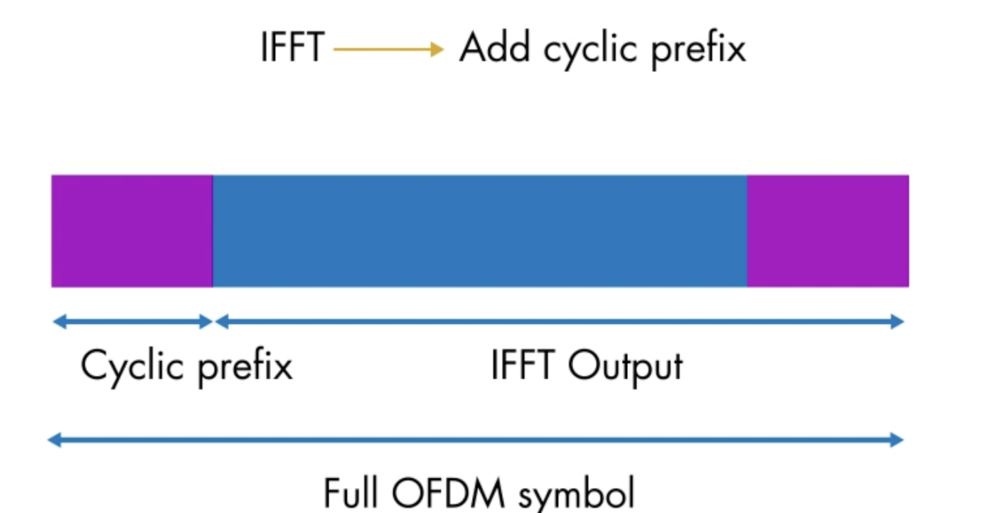
So in the transmitter you have the IFFT output. then you add the cyclic prefix to get a full OFDM symbol,

image-20230910153655301

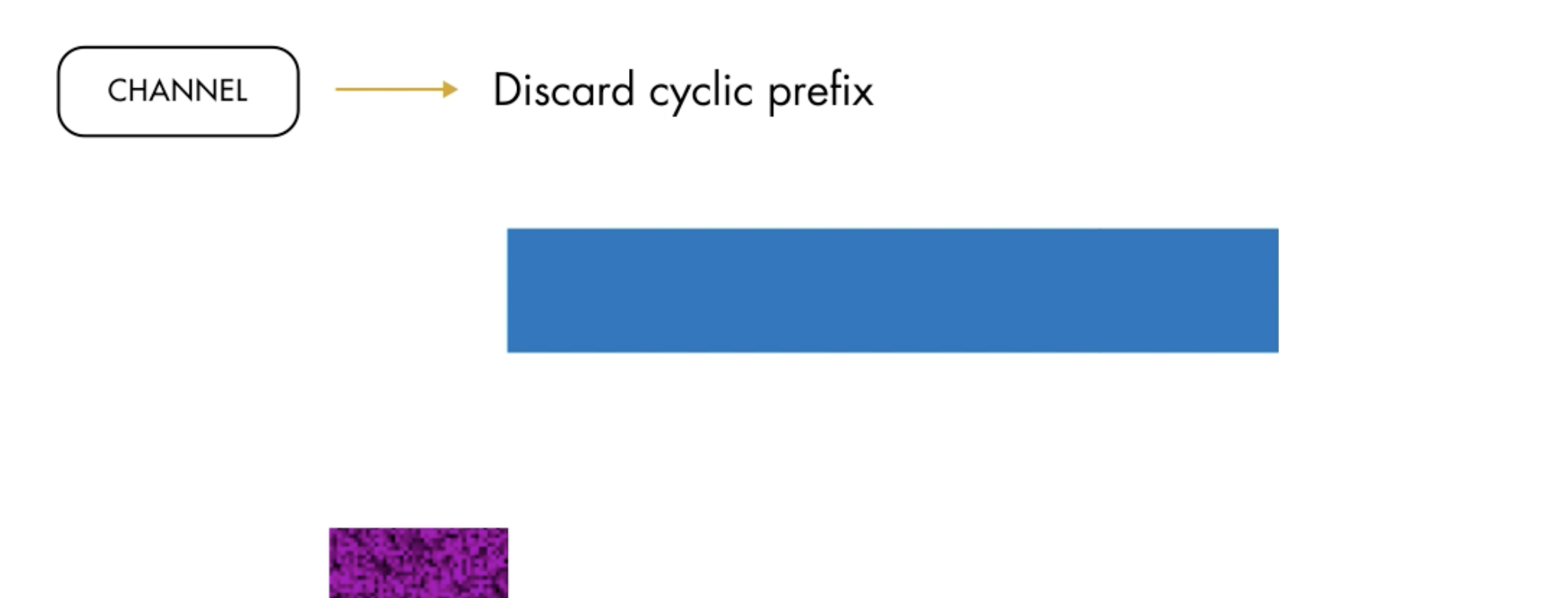
On the other hand, in the receiver, the operation is run in reverse.

First you strip off the cyclic prefix, getting rid of all that multipath corruption.

image-20230910153932708

Then perform FFT,

image-20230910154006082

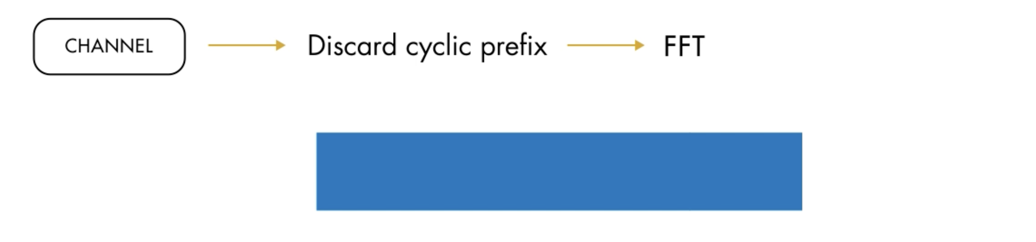
Then you can equalize the signal using that beautiful simple division!

and your output is the QAM signal you start with.

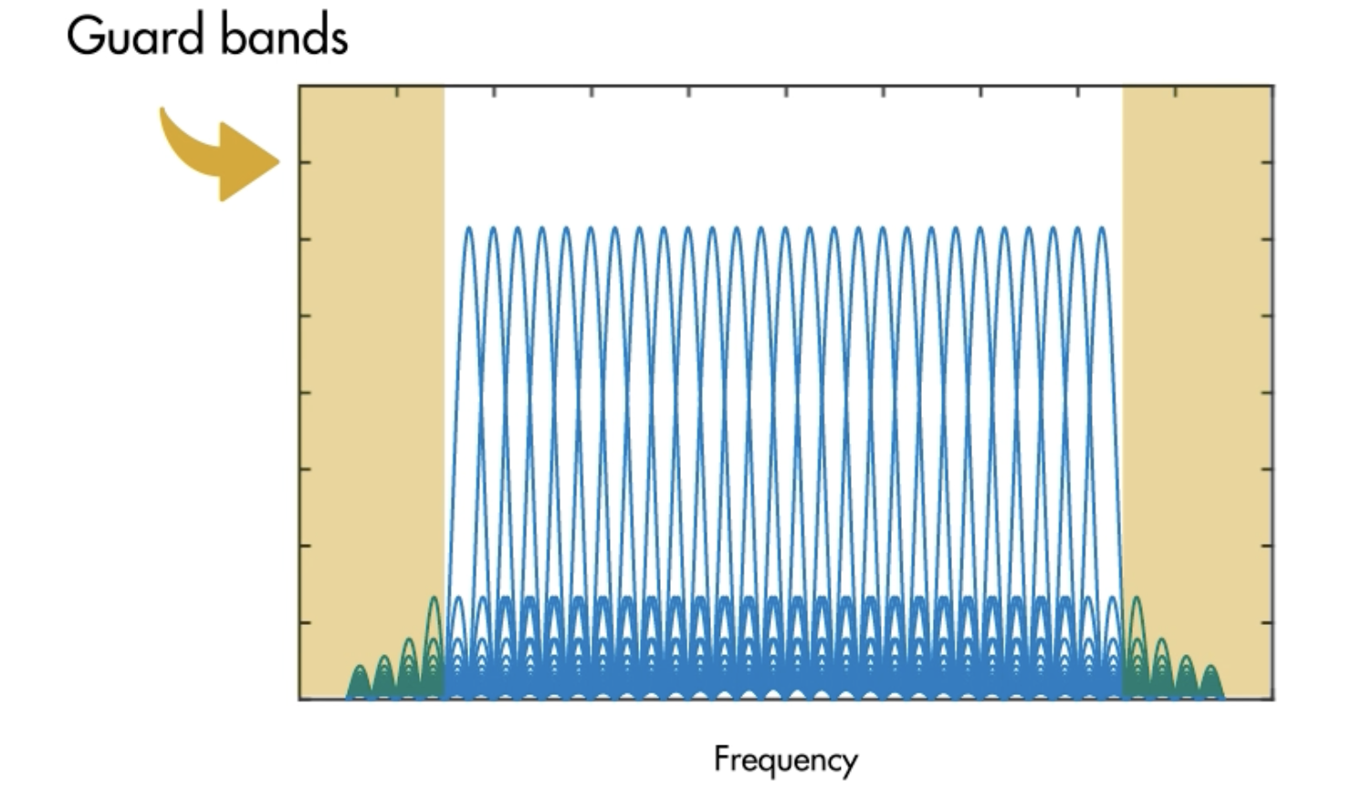
Note: In the OFDM, the guardbands are in the external part the whold bandwidth.

image-20230910154249442

image-20230910154332598

1
2
3
4
5
6
7
8
9
10
11
12
13
14
15
16
17
18
19
20
21
22
23
24
25
26
27
28
29
30
31
32
33
34
35
36
modOrder = 16;
bitsPerSymbol = log2(modOrder);
mpChan = [0.8; zeros(7, 1); -0.5; zeros[7, 1]; 0.34];%multipath channel
SNR = 15;
numCarr = 8192;
numBits = numCarr * bitsPerSymbol;
%the number of bits.

if exist("numBits", "var")
srcBits = randi([0, 1], numBits, 1);
qamModOut = qammod(srcBits, modOrder, "InputType", "bit", "UnitAveragePower", true);
end

cycPrefLen = 32;
%the length of cyclic prefix is at least the same as that of inpulse response, which has the %length 17, 32>17.
ofdmModOut = ofdmmod(qamModOut, numCarr, cycPrefLen);

if exist("ofdmModOut", "var")
mpChanOut = filter(mpChan, 1, ofdmModOut);%the multipath channel is equal to a filter.
chanOut = awgn(mpChanOut, SNR, "measured");
end

ofdmDemodOut = ofdmdemod(chanOut, numCarr, cycPrefLen);%demodulate and delete the prefix
scatterplot(ofdmDemodOut);

%Then use the division!
npChanFreq = fftshift(fft(mpChan, numCarr));%frequency response H
%fft 函数的输出以零频率分量开始,但 ofdmdemod 函数指定的是频率范围中间的零频率分量。使用 fftshift 移动信道的频谱,使零频率分量位于中心。
eqOut = ofdmDemodOut ./ mpChanFreq;
scatterplot(eqOut);
title("Frequency Domain Equalizer Output");
if exist("eqOut", "var")
qamDemodOut = qamdemod(eqOut, modOrder, "OutputType", "bit", "UnitAveragePower", true);
numBitErrors = nnz(srcBits ~= qamDemodOut);
BER = numBitErrors ./ numBits;
end

There are some additional attributions in the OFDM system, such as void subcarriers.
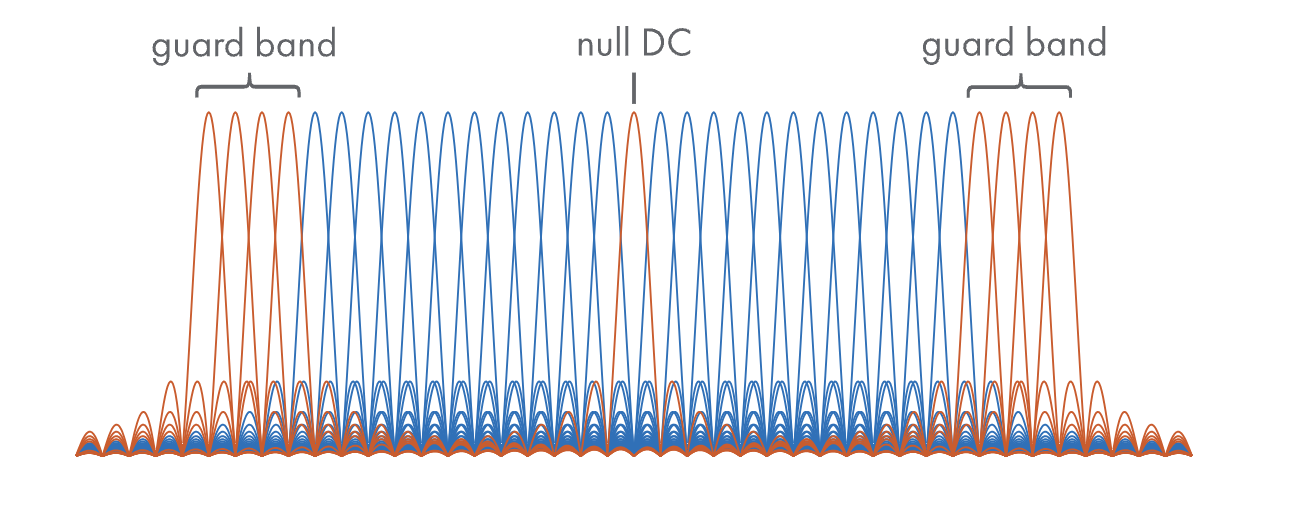
Void subcarriers

People usually distribute guard bands to the lower part of bandwidth and the higher part of bandwidth, to reduce the interference from neighbors. They also give 0 to DC position, to remove the DC signals

image-20230910163842996

1
2
3
4
5
6
7
8
9
10
11
12
13
14
15
16
17
18
19
20
21
22
23
24
25
26
27
28
29
30
31
32
33
34
35
36
37
38
39
40
41
42
43
44
45
46
47
48
49
50
51
52
53
54
55
modOrder = 16;
bitsPerSymbol = log2(modOrder);
mpChan = [0.8; zeros(7, 1); -0.5; zeros(7, 1); 0.34];%multipath channel
SNR = 15;
numCarr = 8192;
cycPrefLen = 32;%cyclic prefix length

numGBCarr = numCarr / 16;
gbLeft = 1:numGBCarr;%safe guard band range, the left frequency part
gbRight = (numCarr - numGBCarr + 1):numCarr;
%定义了左右两端的保护边带

dcIdx = (numCarr / 2) + 1;%the index of the dc band
nullIdx = [gbLeft deIdx gbRight].';
%this is the index of null bands
numDataCarr = numCarr - length(nullIdx);%subtract null bands, remaining the data bands.
numBits = numDataCarr * bitsPerSymbol;%number of bits of data


%modulate
if exist("numBits", "var")
srcBits = randi([0, 1], numBits, 1);
qamModOut = qammod(srcBits, modOrder, "InputType, "bit", "UnitAveragePower", true);
end
ofdmModOut = ofdmmod(qamModOut, numCarr, cycPrefLen, nullIdx);%input null bands index %parameters

%channel part
if exist("ofdmModOut", "var")
mpChanOut = filter(mpChan, 1, ofdmModOut);
chanOut = awgn(mpChanOut, SNR, "measured");
end

ofdmDemodOut = ofdmdemod(chanOut, numCarr, cycPrefLen, cycPrefLen, nullIdx);
%由于使用了空子载波,所以需要两个额外参数,采样偏移量和空索引向量。
%采样偏移量就是执行fft之前丢弃的信号采样数。为0到循环前缀长度之间的任何值,也就是删除掉
%被信道损坏的信息,所以我们直接用前缀长度

%remove equalizer
mpChanOut = fftshift(fft(mpChan, numCarr));%shift dc to the center
%注意,包含了空子载波,因为要进行除法
mpChanOut(nullIdx) = [];%空子载波被移除
eqOut = ofdmDemodOut ./ mpChanOut;
scatterplot(eqOut);

%calculate BER
if exist("eqOut", "var")
qamdemodOut = qamdemod(eqOut, modOrder, "OutputType", "bit", "UnitAveragePower", true);
numBitErrors = nnz(srcBits ~= qamdemodOut);
BER = numBitErrors / numBits;
disp(BER);
end

%draw spectra analyser, draw the ofdm transmitting signal with yellow , and noise contained multipath signal with blue, including safe guard bands and dc band and frequency selecting fading.
specAn = dsp.SpectrumAnalyzer("NumInputPorts", 2, "SpectralAverages", 50, "ShowLegend", true, "ShowGrid", true);
specAn(ofdmModOut, chanOut);

image-20230910191254730

image-20230910191310962